Chapter 5 of 12

Updated 6 August 2026

NCERT Solutions

Production and Costs — NCERT Solutions

Madhya Pradesh Board · Class 12 · Economics

NCERT Solutions for Production and Costs, Madhya Pradesh Board Class 12 Economics: 30 textbook questions solved step by step.

42 questions74 flashcards7 formulas & key relations5 concepts

Interactive on Super Tutor

Studying Production and Costs? Get the full interactive chapter.

Quizzes, flashcards, AI doubt-solver and a step-by-step study plan — built for NCERT solutions and more.

Try Super Tutor — Free

Free trial, no card needed.

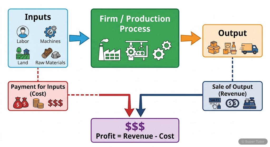
A flowchart illustrating the transformation of various inputs (labor, capital, raw materials) into an output by a firm, highlighting the payment for inputs (cost), sale of output (revenue), and the re — Learn better with visuals Super Tutor pairs illustrations like this with notes and quizzes for Production and Costs.

30 Questions Solved · 1 Section

The first 15 solutions are open to read. The other 15 are free with a Super Tutor account.

Exercises — Production and Costs

1Explain the concept of a production function.Show solution

Given/Concept: A production function describes the technical relationship between inputs and output.

Definition: A production function gives the maximum quantity of output that can be produced from any given combination of inputs, for a given state of technology.

Mathematically, it is written as:
$Q = f(L, K)$
where $Q$ = quantity of output, $L$ = labour, $K$ = capital.

Key points:

It shows all technically efficient combinations of inputs that yield a given level of output.
It is defined for a given technology; if technology improves, the production function itself changes.
It can be studied in the short run (some inputs fixed) and the long run (all inputs variable).

Conclusion: The production function is a fundamental concept that summarises the firm's production technology and helps determine the least-cost method of producing any desired level of output.

2What is the total product of an input?Show solution

Definition: The Total Product (TP) of an input is the total quantity of output produced when a given amount of that input is used, keeping all other inputs constant.

Formula:
$TP_L = f(L, \bar{K})$
where $\bar{K}$ denotes that capital is held fixed.

Explanation:

As more units of the variable input (say, labour) are employed, total product initially increases at an increasing rate, then at a decreasing rate, and may eventually decline.
The total product schedule shows the output corresponding to each level of the variable input.

Example: If 1 worker produces 10 units, 2 workers produce 25 units, and 3 workers produce 35 units, then $TP$ at $L=1$ is 10, at $L=2$ is 25, and at $L=3$ is 35.

3What is the average product of an input?Show solution

Definition: The Average Product (AP) of an input is the output produced per unit of the variable input employed.

Formula:
$AP_L = \frac{TP_L}{L}$
where $TP_L$ = total product of labour and $L$ = number of units of labour employed.

Behaviour:

The AP curve is inverse U-shaped: it first rises, reaches a maximum, and then falls.
AP rises as long as each additional worker contributes more than the average, and falls when each additional worker contributes less than the average.

Example: If $TP = 30$ when $L = 3$ , then $AP_L = \frac{30}{3} = 10$ units per worker.

4What is the marginal product of an input?Show solution

Definition: The Marginal Product (MP) of an input is the additional output produced when one more unit of that input is employed, keeping all other inputs constant.

Formula:
$MP_L = TP_L(n) - TP_L(n-1)$
or in calculus notation:
$MP_L = \frac{\Delta TP_L}{\Delta L}$

Behaviour:

The MP curve is also inverse U-shaped.
MP first increases (increasing returns to the variable factor), then decreases (diminishing returns), and may become negative.

Example: If $TP$ at $L=3$ is 50 and $TP$ at $L=2$ is 35, then $MP$ at $L=3$ is $50 - 35 = 15$ units.

5Explain the relationship between the marginal products and the total product of an input.Show solution

Concept: The total product is the sum of all marginal products up to that level of employment.

Mathematical Relationship:
$TP_L(n) = \sum_{i=1}^{n} MP_L(i) = MP_L(1) + MP_L(2) + \cdots + MP_L(n)$

Graphical Relationship:

When MP > 0: TP is increasing. Each additional unit of labour adds to total output.
When MP is rising: TP increases at an increasing rate (convex shape).
When MP is falling but positive: TP increases at a decreasing rate (concave shape).
When MP = 0: TP is at its maximum.
When MP < 0: TP starts declining.

Conclusion: The MP curve intersects the horizontal axis exactly at the point where TP reaches its maximum. The area under the MP curve up to any level of labour gives the total product at that level.

6Explain the concepts of the short run and the long run.Show solution

Short Run:

The short run is a period of time in which at least one input is fixed and cannot be varied.
Typically, capital (plant and machinery) is the fixed input, while labour is the variable input.
The firm can change its output only by changing the variable input.
Example: A factory cannot immediately build a new plant; it can only hire more workers.

Long Run:

The long run is a period of time in which all inputs can be varied.
There are no fixed inputs in the long run; the firm can change its scale of production entirely.
The firm can choose the optimal combination of all inputs.
Example: In the long run, a firm can expand its factory, install new machinery, and hire more workers.

Key Distinction: The short run and long run are not defined by a specific calendar time period; they depend on the nature of the industry. For some industries, the long run may be a few months; for others, it may be several years.

7What is the law of diminishing marginal product?Show solution

Statement: The Law of Diminishing Marginal Product states that as more and more units of a variable input are employed, keeping other inputs fixed, the marginal product of the variable input eventually decreases.

Explanation:

Initially, when more units of the variable input (e.g., labour) are added to a fixed input (e.g., capital), the marginal product may increase due to better utilisation of the fixed factor.
However, beyond a certain point, the fixed factor becomes a constraint, and each additional unit of the variable input adds less and less to total output.
Eventually, MP may even become zero or negative.

Example: In a factory with fixed machinery, adding the 1st worker may produce 10 units, the 2nd worker 15 units (MP rises), but the 5th worker may add only 5 units (MP falls) because the machinery is being overused.

Conclusion: This law operates in the short run when at least one input is fixed.

8What is the law of variable proportions?Show solution

Statement: The Law of Variable Proportions states that as the proportion of one variable input is increased relative to other fixed inputs, the total product first increases at an increasing rate, then at a decreasing rate, and finally decreases.

Three Stages:

Stage	Behaviour of MP	Behaviour of TP
Stage I	MP rises (MP > AP)	TP increases at increasing rate
Stage II	MP falls but MP > 0	TP increases at decreasing rate
Stage III	MP < 0	TP decreases

Reason: As more of the variable input is added to a fixed input, the ratio of variable to fixed input changes. Initially, the fixed factor is underutilised, so adding variable input improves efficiency. Beyond a point, the fixed factor becomes a bottleneck.

Relationship with Diminishing Marginal Product: The law of variable proportions is a broader statement; the law of diminishing marginal product refers specifically to Stage II and beyond.

Conclusion: A rational firm will always operate in Stage II, where both AP and MP are positive but declining.

9When does a production function satisfy constant returns to scale?Show solution

Definition: A production function exhibits Constant Returns to Scale (CRS) when a proportionate increase in all inputs leads to an equal proportionate increase in output.

Condition: If all inputs are multiplied by a constant factor $\lambda > 1$ , and output also increases by the same factor $\lambda$ , then the production function shows CRS.

Mathematically:
$f(\lambda L, \lambda K) = \lambda \cdot f(L, K) = \lambda Q$

Example: If a firm doubles both labour and capital (i.e., $\lambda = 2$ ) and output also doubles, the production function satisfies CRS.

Reason: CRS occurs when the gains from specialisation and division of labour are exactly offset by the difficulties of managing a larger scale of operation.

10When does a production function satisfy increasing returns to scale?Show solution

Definition: A production function exhibits Increasing Returns to Scale (IRS) when a proportionate increase in all inputs leads to a more than proportionate increase in output.

Condition: If all inputs are multiplied by $\lambda > 1$ and output increases by more than $\lambda$ , then the production function shows IRS.

Mathematically:
$f(\lambda L, \lambda K) > \lambda \cdot f(L, K)$

Example: If a firm doubles both labour and capital and output more than doubles (say, triples), the production function satisfies IRS.

Reasons for IRS:

Greater specialisation and division of labour at larger scales.
Technical advantages of large-scale production.
Indivisibility of certain inputs (e.g., a machine cannot be used at half capacity efficiently).

11When does a production function satisfy decreasing returns to scale?Show solution

Definition: A production function exhibits Decreasing Returns to Scale (DRS) when a proportionate increase in all inputs leads to a less than proportionate increase in output.

Condition: If all inputs are multiplied by $\lambda > 1$ and output increases by less than $\lambda$ , then the production function shows DRS.

Mathematically:
$f(\lambda L, \lambda K) < \lambda \cdot f(L, K)$

Example: If a firm doubles both labour and capital but output increases by only 50% (less than doubles), the production function satisfies DRS.

Reasons for DRS:

Difficulties in managing and coordinating a very large organisation.
Managerial inefficiencies at large scales.
Scarcity of specialised inputs that cannot be increased proportionately.

12Briefly explain the concept of the cost function.Show solution

Definition: A cost function shows the minimum cost of producing any given level of output, given the prices of inputs and the production technology.

Mathematical Form:
$C = f(Q, w, r)$
where $C$ = total cost, $Q$ = quantity of output, $w$ = wage rate (price of labour), $r$ = rental rate (price of capital).

Key Points:

The cost function is derived from the production function by choosing the least-cost combination of inputs for each level of output.
In the short run, the cost function has both fixed and variable components because some inputs are fixed.
In the long run, all costs are variable since all inputs can be changed.
The cost function helps the firm decide how much to produce and what combination of inputs to use.

Conclusion: The cost function is the monetary counterpart of the production function and is essential for profit maximisation decisions.

13What are the total fixed cost, total variable cost and total cost of a firm? How are they related?Show solution

Total Fixed Cost (TFC):

TFC is the cost incurred on fixed inputs (e.g., rent, insurance, depreciation on machinery).
It does not change with the level of output; it remains constant even when output is zero.
Example: Monthly rent of a factory = Rs 10,000 regardless of production.

Total Variable Cost (TVC):

TVC is the cost incurred on variable inputs (e.g., wages of daily workers, raw materials).
It changes with the level of output: TVC = 0 when Q = 0, and it increases as output increases.
Example: Cost of raw materials increases as more units are produced.

Total Cost (TC):

TC is the total expenditure incurred by the firm on all inputs (fixed + variable) to produce a given level of output.

Relationship:
$TC = TFC + TVC$

Graphically:

The TFC curve is a horizontal straight line (parallel to the output axis).
The TVC curve starts from the origin and rises with output.
The TC curve is obtained by adding TFC vertically to the TVC curve; it starts from the point on the Y-axis equal to TFC.

14What are the average fixed cost, average variable cost and average cost of a firm? How are they related?Show solution

Average Fixed Cost (AFC):
$AFC = \frac{TFC}{Q}$

AFC is the fixed cost per unit of output. Since TFC is constant, AFC falls continuously as output increases (rectangular hyperbola shape).

Average Variable Cost (AVC):
$AVC = \frac{TVC}{Q}$

AVC is the variable cost per unit of output. The AVC curve is U-shaped: it first falls, reaches a minimum, and then rises.

Average Cost / Short Run Average Cost (SAC):
$SAC = \frac{TC}{Q}$

SAC is the total cost per unit of output. The SAC curve is also U-shaped.

Relationship:
$SAC = AFC + AVC$

Derivation:
$SAC = \frac{TC}{Q} = \frac{TFC + TVC}{Q} = \frac{TFC}{Q} + \frac{TVC}{Q} = AFC + AVC$

Graphically: The vertical distance between the SAC curve and the AVC curve equals AFC at every level of output. As output increases, this distance narrows because AFC falls continuously.

15Can there be some fixed cost in the long run? If not, why?Show solution

Answer: No, there cannot be any fixed cost in the long run.

Reason:

In the long run, by definition, all inputs are variable. The firm has sufficient time to adjust all factors of production — labour, capital, land, etc.
Since no input is fixed in the long run, there is no cost that remains constant regardless of output.
The firm can expand or contract its entire scale of operations, including its plant size, machinery, and workforce.
Therefore, all costs in the long run are variable costs.

Implication:
$TC_{LR} = TVC_{LR}$
and
$AFC_{LR} = 0$

Conclusion: Fixed costs are a short-run phenomenon arising from the existence of fixed inputs. In the long run, since the firm can vary all inputs, every cost becomes a variable cost.

16What does the average fixed cost curve look like? Why does it look so?

Shape: The Average Fixed Cost (AFC) curve is a downward sloping rectangular hyperbola.

Formula:
$AFC = \frac{TFC}{Q}$

Why it looks so:

TFC is a constant (say, Rs $C$ ). Therefore, $AFC = \frac{C}{Q}$ .
As output $Q$ increases, AFC continuously decreases but never becomes zero (it approaches zero asymptotically).
This is because a fixed total amount (TFC) is being spread over more and more units of output.
The product $AFC \times Q = TFC =$ constant, which is the equation of a rectangular hyperbola.

Key Properties:

AFC is always positive and always declining.
It never touches the X-axis (AFC → 0 as Q → ∞).
It never touches the Y-axis (AFC → ∞ as Q → 0).
The area under the AFC curve at any output level equals TFC.

Conclusion: The AFC curve is a rectangular hyperbola because a fixed total cost is divided by an ever-increasing quantity of output.

Free with a Super Tutor account

17What do the short run marginal cost, average variable cost and short run average cost curves look like?

Shape of all three curves: All three — SMC, AVC, and SAC — are U-shaped.

Short Run Marginal Cost (SMC):

SMC first falls as output increases (due to increasing returns to the variable factor).
It reaches a minimum and then rises (due to diminishing returns to the variable factor).
The SMC curve is U-shaped and is the steepest of the three.

Average Variable Cost (AVC):

AVC first falls, reaches a minimum, and then rises — giving a U-shape.
The minimum of AVC occurs to the right of the minimum of SMC.
SMC cuts AVC at its minimum point from below.

Short Run Average Cost (SAC):

SAC = AFC + AVC. Since AFC is always falling, SAC falls more steeply than AVC initially.
SAC reaches its minimum at a higher output level than AVC.
SMC cuts SAC at its minimum point from below.

Relative Positions:

The SMC curve lies below both AVC and SAC when they are falling, and above both when they are rising.
The minimum of SMC < minimum of AVC < minimum of SAC (in terms of output levels).
At low output levels, SAC > AVC (the gap = AFC); as output rises, the gap narrows.

Free with a Super Tutor account

18Why does the SMC curve cut the AVC curve at the minimum point of the AVC curve?

Concept: This follows from the mathematical relationship between marginal and average values.

Proof/Reasoning:

We know:
$AVC = \frac{TVC}{Q}$

For AVC to be at its minimum, its rate of change must be zero:
$\frac{d(AVC)}{dQ} = 0$

$\frac{d}{dQ}\left(\frac{TVC}{Q}\right) = \frac{Q \cdot \frac{d(TVC)}{dQ} - TVC}{Q^2} = 0$

$\Rightarrow Q \cdot SMC - TVC = 0$

$\Rightarrow SMC = \frac{TVC}{Q} = AVC$

Intuitive Explanation:

When SMC < AVC: Each additional unit costs less than the average, so AVC is being pulled down → AVC is falling.
When SMC > AVC: Each additional unit costs more than the average, so AVC is being pulled up → AVC is rising.
Therefore, AVC is at its minimum exactly when SMC = AVC, i.e., the SMC curve cuts the AVC curve at the minimum point of AVC.

Conclusion: The SMC curve must pass through the minimum point of the AVC curve — it cuts AVC from below at that point.

Free with a Super Tutor account

19At which point does the SMC curve cut the SAC curve? Give reason in support of your answer.

Answer: The SMC curve cuts the SAC curve at the minimum point of the SAC curve.

Reason (Mathematical):

We know:
$SAC = \frac{TC}{Q}$

At the minimum of SAC:
$\frac{d(SAC)}{dQ} = 0$

$\frac{d}{dQ}\left(\frac{TC}{Q}\right) = \frac{Q \cdot \frac{d(TC)}{dQ} - TC}{Q^2} = 0$

$\Rightarrow Q \cdot SMC - TC = 0$

$\Rightarrow SMC = \frac{TC}{Q} = SAC$

Intuitive Explanation:

When SMC < SAC: The marginal cost is less than the average total cost, pulling SAC downward → SAC is falling.
When SMC > SAC: The marginal cost exceeds the average total cost, pulling SAC upward → SAC is rising.
Therefore, SAC is at its minimum when SMC = SAC.

Conclusion: The SMC curve cuts the SAC curve from below at the minimum point of the SAC curve, for the same reason that any marginal curve cuts its corresponding average curve at the average's minimum point.

Free with a Super Tutor account

20Why is the short run marginal cost curve 'U'-shaped?

Answer: The SMC curve is U-shaped because of the Law of Variable Proportions (or the Law of Diminishing Marginal Product).

Explanation:

$SMC = \frac{\Delta TC}{\Delta Q} = \frac{\Delta TVC}{\Delta Q} = \frac{w \cdot \Delta L}{\Delta Q} = \frac{w}{MP_L}$

where $w$ = wage rate (assumed constant) and $MP_L$ = marginal product of labour.

Stage 1 — Falling SMC:

Initially, as more labour is employed, $MP_L$ rises (increasing returns to the variable factor).
Since $SMC = \frac{w}{MP_L}$ , as $MP_L$ rises, SMC falls.
This is because each additional worker is more productive than the previous one.

Stage 2 — Rising SMC:

Beyond a certain point, due to the Law of Diminishing Marginal Product, $MP_L$ starts to fall.
As $MP_L$ falls, $SMC = \frac{w}{MP_L}$ rises.
Each additional unit of output requires more and more labour (and hence more cost).

Conclusion: Since $MP_L$ first rises and then falls (inverse U-shape), SMC first falls and then rises, giving it a U-shape. The minimum of SMC corresponds to the maximum of $MP_L$ .

Free with a Super Tutor account

21What do the long run marginal cost and the average cost curves look like?

Shape: Both the Long Run Average Cost (LRAC) curve and the Long Run Marginal Cost (LRMC) curve are U-shaped.

Long Run Average Cost (LRAC):

The LRAC curve is also called the 'envelope curve' or 'planning curve' because it is the lower envelope of all the short run average cost (SAC) curves.
It is U-shaped due to returns to scale:
Falling portion: Due to Increasing Returns to Scale (economies of scale) — as output expands, LRAC falls.
Minimum point: Constant Returns to Scale.
Rising portion: Due to Decreasing Returns to Scale (diseconomies of scale) — as output expands further, LRAC rises.

Long Run Marginal Cost (LRMC):

The LRMC curve is also U-shaped.
It lies below LRAC when LRAC is falling and above LRAC when LRAC is rising.
LRMC cuts LRAC at the minimum point of LRAC from below.

Key Difference from Short Run:

The U-shape of LRAC is due to returns to scale (a long-run concept), whereas the U-shape of SAC is due to the law of variable proportions (a short-run concept).
The LRAC curve is flatter and wider than the SAC curves.

Conclusion: Both LRAC and LRMC are U-shaped, with LRMC cutting LRAC at its minimum point from below.

Free with a Super Tutor account

22The following table gives the total product schedule of labour. Find the corresponding average product and marginal product schedules of labour.

| L | TPL |
|---|---|
| 0 | 0 |
| 1 | 15 |
| 2 | 35 |
| 3 | 50 |
| 4 | 40 |
| 5 | 48 |

Given: Total Product schedule of labour.

Formulae:
$AP_L = \frac{TP_L}{L}$
$MP_L = TP_L(n) - TP_L(n-1)$

Calculations:

At L = 1:
$AP_L = \frac{15}{1} = 15$
$MP_L = 15 - 0 = 15$

At L = 2:
$AP_L = \frac{35}{2} = 17.5$
$MP_L = 35 - 15 = 20$

At L = 3:
$AP_L = \frac{50}{3} = 16.67$
$MP_L = 50 - 35 = 15$

At L = 4:
$AP_L = \frac{40}{4} = 10$
$MP_L = 40 - 50 = -10$

At L = 5:
$AP_L = \frac{48}{5} = 9.6$
$MP_L = 48 - 40 = 8$

Complete Schedule:

L	$TP_L$	$AP_L$	$MP_L$
0	0	—	—
1	15	15	15
2	35	17.5	20
3	50	16.67	15
4	40	10	−10
5	48	9.6	8

Note: At L = 4, MP is negative (−10), meaning the 4th worker actually reduces total output. This is Stage III of the Law of Variable Proportions.

Free with a Super Tutor account

23The following table gives the average product schedule of labour. Find the total product and marginal product schedules. It is given that the total product is zero at zero level of labour employment.

| L | APL |
|---|---|
| 1 | 2 |
| 2 | 3 |
| 3 | 4 |
| 4 | 4.25 |
| 5 | 4 |
| 6 | 3.5 |

Given: $AP_L$ schedule; $TP_L = 0$ at $L = 0$ .

Formula for TP:
$TP_L = AP_L \times L$

Formula for MP:
$MP_L(n) = TP_L(n) - TP_L(n-1)$

Calculations:

At L = 1: $TP = 2 \times 1 = 2$ ; $MP = 2 - 0 = 2$

At L = 2: $TP = 3 \times 2 = 6$ ; $MP = 6 - 2 = 4$

At L = 3: $TP = 4 \times 3 = 12$ ; $MP = 12 - 6 = 6$

At L = 4: $TP = 4.25 \times 4 = 17$ ; $MP = 17 - 12 = 5$

At L = 5: $TP = 4 \times 5 = 20$ ; $MP = 20 - 17 = 3$

At L = 6: $TP = 3.5 \times 6 = 21$ ; $MP = 21 - 20 = 1$

Complete Schedule:

L	$AP_L$	$TP_L$	$MP_L$
0	—	0	—
1	2	2	2
2	3	6	4
3	4	12	6
4	4.25	17	5
5	4	20	3
6	3.5	21	1

Free with a Super Tutor account

24The following table gives the marginal product schedule of labour. It is also given that total product of labour is zero at zero level of employment. Calculate the total and average product schedules of labour.

| L | MPL |
|---|---|
| 1 | 3 |
| 2 | 5 |
| 3 | 7 |
| 4 | 5 |
| 5 | 3 |
| 6 | 1 |

Given: $MP_L$ schedule; $TP_L = 0$ at $L = 0$ .

Formula for TP:
$TP_L(n) = TP_L(n-1) + MP_L(n)$
(i.e., TP is the cumulative sum of MP)

Formula for AP:
$AP_L = \frac{TP_L}{L}$

Calculations:

At L = 1: $TP = 0 + 3 = 3$ ; $AP = \frac{3}{1} = 3$

At L = 2: $TP = 3 + 5 = 8$ ; $AP = \frac{8}{2} = 4$

At L = 3: $TP = 8 + 7 = 15$ ; $AP = \frac{15}{3} = 5$

At L = 4: $TP = 15 + 5 = 20$ ; $AP = \frac{20}{4} = 5$

At L = 5: $TP = 20 + 3 = 23$ ; $AP = \frac{23}{5} = 4.6$

At L = 6: $TP = 23 + 1 = 24$ ; $AP = \frac{24}{6} = 4$

Complete Schedule:

L	$MP_L$	$TP_L$	$AP_L$
0	—	0	—
1	3	3	3
2	5	8	4
3	7	15	5
4	5	20	5
5	3	23	4.6
6	1	24	4

Free with a Super Tutor account

25The following table shows the total cost schedule of a firm. What is the total fixed cost schedule of this firm? Calculate the TVC, AFC, AVC, SAC and SMC schedules of the firm.

| Q | TC |
|---|---|
| 0 | 10 |
| 1 | 30 |
| 2 | 45 |
| 3 | 55 |
| 4 | 70 |
| 5 | 90 |
| 6 | 120 |

Step 1: Find TFC
When $Q = 0$ , $TC = TFC$ (since $TVC = 0$ at zero output).
$TFC = 10 \text{ (constant for all Q)}$

Step 2: Find TVC
$TVC = TC - TFC$

Step 3: Find AFC, AVC, SAC
$AFC = \frac{TFC}{Q}, \quad AVC = \frac{TVC}{Q}, \quad SAC = \frac{TC}{Q}$

Step 4: Find SMC
$SMC = TC(Q) - TC(Q-1)$

Complete Schedule:

Q	TC	TFC	TVC	AFC	AVC	SAC	SMC
0	10	10	0	—	—	—	—
1	30	10	20	10	20	30	20
2	45	10	35	5	17.5	22.5	15
3	55	10	45	3.33	15	18.33	10
4	70	10	60	2.5	15	17.5	15
5	90	10	80	2	16	18	20
6	120	10	110	1.67	18.33	20	30

Verification: $SAC = AFC + AVC$ at each level. For example, at $Q=3$ : $3.33 + 15 = 18.33$ ✓

Observation: SMC is minimum at $Q=3$ (SMC = 10), AVC is minimum at $Q=3$ and $Q=4$ (AVC = 15), and SAC is minimum at $Q=4$ (SAC = 17.5). SMC cuts AVC at its minimum (both equal 15 at $Q=4$ ) and cuts SAC at its minimum.

Free with a Super Tutor account

26The following table gives the total cost schedule of a firm. It is also given that the average fixed cost at 4 units of output is Rs 5. Find the TVC, TFC, AVC, AFC, SAC and SMC schedules of the firm for the corresponding values of output.

| Q | TC |
|---|---|
| 1 | 50 |
| 2 | 65 |
| 3 | 75 |
| 4 | 95 |
| 5 | 130 |
| 6 | 185 |

Step 1: Find TFC
Given: $AFC$ at $Q = 4$ is Rs 5.
$TFC = AFC \times Q = 5 \times 4 = Rs\ 20$
TFC is constant at Rs 20 for all output levels.

Step 2: Find TVC
$TVC = TC - TFC$

Step 3: Find AFC, AVC, SAC
$AFC = \frac{TFC}{Q} = \frac{20}{Q}$
$AVC = \frac{TVC}{Q}$
$SAC = \frac{TC}{Q}$

Step 4: Find SMC
$SMC(Q) = TC(Q) - TC(Q-1)$
(Note: TC at Q=0 = TFC = 20, since TVC=0 at Q=0)

Calculations:

Q	TC	TFC	TVC	AFC	AVC	SAC	SMC
1	50	20	30	20	30	50	30
2	65	20	45	10	22.5	32.5	15
3	75	20	55	6.67	18.33	25	10
4	95	20	75	5	18.75	23.75	20
5	130	20	110	4	22	26	35
6	185	20	165	3.33	27.5	30.83	55

Note for SMC at Q=1: $TC(Q=0) = TFC = 20$ , so $SMC(1) = 50 - 20 = 30$ .

Verification at Q=4: $AFC = 5$ ✓; $SAC = AFC + AVC = 5 + 18.75 = 23.75$ ✓

Free with a Super Tutor account

27A firm's SMC schedule is shown in the following table. The total fixed cost of the firm is Rs 100. Find the TVC, TC, AVC and SAC schedules of the firm.

| Q | SMC |
|---|---|
| 0 | — |
| 1 | 500 |
| 2 | 300 |
| 3 | 200 |
| 4 | 300 |
| 5 | 500 |
| 6 | 800 |

Given: TFC = Rs 100; SMC schedule as above.

Step 1: Find TVC
TVC is the cumulative sum of SMC (since TVC = 0 at Q = 0):
$TVC(Q) = \sum_{i=1}^{Q} SMC(i)$

Step 2: Find TC
$TC = TFC + TVC = 100 + TVC$

Step 3: Find AVC and SAC
$AVC = \frac{TVC}{Q}, \quad SAC = \frac{TC}{Q}$

Calculations:

At Q = 0: $TVC = 0$ ; $TC = 100$

At Q = 1: $TVC = 500$ ; $TC = 600$ ; $AVC = 500$ ; $SAC = 600$

At Q = 2: $TVC = 500 + 300 = 800$ ; $TC = 900$ ; $AVC = \frac{800}{2} = 400$ ; $SAC = \frac{900}{2} = 450$

At Q = 3: $TVC = 800 + 200 = 1000$ ; $TC = 1100$ ; $AVC = \frac{1000}{3} = 333.33$ ; $SAC = \frac{1100}{3} = 366.67$

At Q = 4: $TVC = 1000 + 300 = 1300$ ; $TC = 1400$ ; $AVC = \frac{1300}{4} = 325$ ; $SAC = \frac{1400}{4} = 350$

At Q = 5: $TVC = 1300 + 500 = 1800$ ; $TC = 1900$ ; $AVC = \frac{1800}{5} = 360$ ; $SAC = \frac{1900}{5} = 380$

At Q = 6: $TVC = 1800 + 800 = 2600$ ; $TC = 2700$ ; $AVC = \frac{2600}{6} = 433.33$ ; $SAC = \frac{2700}{6} = 450$

Complete Schedule:

Q	SMC	TVC	TC	AVC	SAC
0	—	0	100	—	—
1	500	500	600	500	600
2	300	800	900	400	450
3	200	1000	1100	333.33	366.67
4	300	1300	1400	325	350
5	500	1800	1900	360	380
6	800	2600	2700	433.33	450

Observation: AVC is minimum at Q = 4 (AVC = 325), and SMC = 300 at Q = 4 which is less than AVC = 325, while SMC = 500 at Q = 5 which is greater than AVC = 360. This confirms SMC cuts AVC at its minimum.

Free with a Super Tutor account

28Let the production function of a firm be

Q = 5L^{\frac{1}{2}}K^{\frac{1}{2}}

. Find out the maximum possible output that the firm can produce with 100 units of

L

and 100 units of

K

Given:

Production function: $Q = 5L^{\frac{1}{2}}K^{\frac{1}{2}}$
$L = 100$ units
$K = 100$ units

Substituting the values:
$Q = 5 \times (100)^{\frac{1}{2}} \times (100)^{\frac{1}{2}}$

$Q = 5 \times 10 \times 10$

$Q = 5 \times 100$

$\boxed{Q = 500 \text{ units}}$

Conclusion: The maximum possible output that the firm can produce with 100 units of labour and 100 units of capital is 500 units.

Free with a Super Tutor account

29Let the production function of a firm be

Q = 2L^{2}K^{2}

. Find out the maximum possible output that the firm can produce with 5 units of

L

and 2 units of

K

. What is the maximum possible output that the firm can produce with zero unit of

L

and 10 units of

K

Given: Production function: $Q = 2L^{2}K^{2}$

Part (i): L = 5, K = 2

$Q = 2 \times (5)^{2} \times (2)^{2}$

$Q = 2 \times 25 \times 4$

$Q = 2 \times 100$

$\boxed{Q = 200 \text{ units}}$

Part (ii): L = 0, K = 10

$Q = 2 \times (0)^{2} \times (10)^{2}$

$Q = 2 \times 0 \times 100$

$\boxed{Q = 0 \text{ units}}$

Conclusion:

With 5 units of L and 2 units of K, the maximum output is 200 units.
With 0 units of L and 10 units of K, the maximum output is 0 units. This is because both inputs are essential (multiplicative production function); if either input is zero, no output can be produced.

Free with a Super Tutor account

30Find out the maximum possible output for a firm with zero unit of

L

and 10 units of

K

when its production function is

Q = 5L + 2K

Given:

Production function: $Q = 5L + 2K$
$L = 0$ units
$K = 10$ units

Substituting the values:
$Q = 5 \times 0 + 2 \times 10$

$Q = 0 + 20$

$\boxed{Q = 20 \text{ units}}$

Conclusion: The maximum possible output with zero units of labour and 10 units of capital is 20 units.

Note: Unlike the multiplicative production function in Q.29, this is an additive (linear) production function. Here, labour and capital are perfect substitutes — production is possible even if one input is zero, as long as the other input is available. Hence, even with no labour, the firm can produce 20 units using only capital.

Free with a Super Tutor account

15 more solved questions in Production and Costs

They are free with a Super Tutor account, along with practice quizzes and flashcards for this chapter. Free to start, no card needed.

Frequently Asked Questions

What are the important topics in Production and Costs for Madhya Pradesh Board Class 12 Economics?

Key topics in Production and Costs include Production Function and Isoquants, Short Run, Long Run, TP, AP and MP, Law of Variable Proportions and Curve Shapes, Returns to Scale and Cobb-Douglas Production Function. Study these first, then practise questions on each for the Madhya Pradesh Board Class 12 board exam.

Are these NCERT Solutions for Production and Costs free?

The first 15 of the 30 solutions on this page are open to read. The other 15 are free with a Super Tutor account — signing up is free and needs no card.

How should I revise Production and Costs for the Madhya Pradesh Board Class 12 board exam?

Learn the core ideas first, then work through the 42 practice questions on Production and Costs. Revise definitions regularly and use flashcards for quick recall before the exam.

Sources & Official References

Content is aligned to the official syllabus. Refer to the board website for the latest curriculum.

More resources for Production and Costs

All Madhya Pradesh Board Class 12 Economics NCERT Solutions

For serious students

Get the full Production and Costs chapter — start free.

Quizzes, flashcards, an AI doubt solver and a study plan for Madhya Pradesh Board Class 12 Economics. Free to start, no card needed.

Try Super Tutor Free

Try this chapter free

Production and Costs — NCERT Solutions

Studying Production and Costs? Get the full interactive chapter.

Exercises — Production and Costs

Frequently Asked Questions

Sources & Official References

More resources for Production and Costs

Practice Quiz

Important Questions

Revision Notes

Formula Sheet

Chapter Summary

Concept Maps

Study Plan

Flashcards

Syllabus

Get the full Production and Costs chapter — start free.